I have this unquenchable fascination for knowing what is going to happen next.
How many visitors are likely to visit my site next week, given I know the history of visits? So that I provision few more computing machines.
What are the best possible action items I can suggest to my team next week, given I know their context? So that the team reaches the next potential point of execution and I prepare myself for the forthcoming coaching sessions.
Your guess is correct. It is going to be one more post on Bayesian inference and probabilistic programming.
A common pattern to model inference cases starts with deciding a suitable probability distribution to represent our observed data and its context.
We use the Poisson distribution to model the number of events emitted at a constant unit of time. For example, the number of visitors visiting a store every day can be modeled with a Poisson distribution with a rate parameter denoted as Lambda.
In another scenario, we choose a Gamma distribution to model the average rain-fall in a month, and the average load on the Web Server in a day.
For our discussion, let us create a Gamma Distribution by directly specifying the parameters a = 2 and b = 2. Let us call these two parameters as the shape and scale of the distribution.

But in reality, the parameters are difficult to determine because our observations are never large enough and they are just a representation of actual data.
For example, if our observation is just a 100 random data from the above sample space, the estimation of the parameters is just an approximation with a high degree of uncertainty.
Markov Chain Monte Carlo is a family of algorithms to discover the hidden parameters that works the way we play the right-ah-right Pandi Game.
For the interest of time here is my futile attempt to explain the MCMC in plain English without resorting to any mathematical equation. Trust me the rust code, we are going to write, will explain the concept better even if you are new to Rust.
MCMC uses a Starting Point and two sets of distribution for approximately discovering these hidden parameters. A Proposal Distribution and a Likelihood distribution.
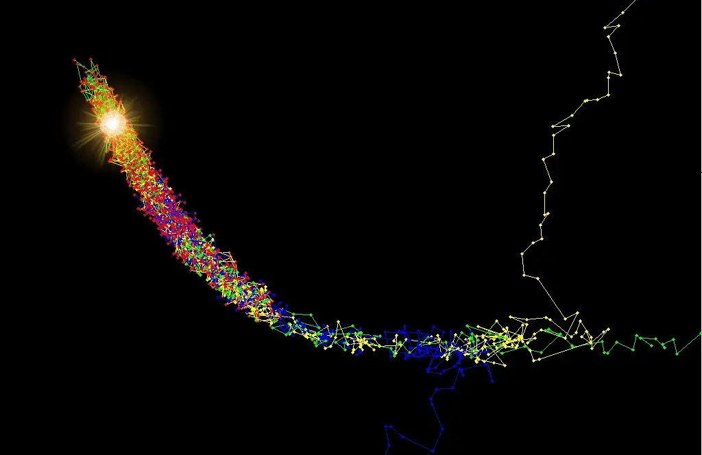
The algorithm does a random walk on the problem space by drawing random sample parameters using the Proposal distribution. An alternate litratature for this activity is the Transition Modeling.
The Likelihood distribution will be used for computing the likelihood value conditional on the observed data.
The computed likelihood will be compared with the current likelihood. The new proposal will be either accepted or rejected by tossing a coin even if the new proposal is unlikely. This will help us to transition to a new region in the proposal distribution. The literature calls this style of walk as the Memory Less Markov because the next point is selected by using just the current point and is not decided by the history of points traveled by the algorithm. The tossing of coin to accept the new proposal is the Monte Carlo Part. Hence the name MCMC
A histogram of the accepted samples will be built with Bins to help us understand the probability of the parameters
Please note that MCMC offers the best possible approximation to the actual parameters.
Ok Fine, what is next?
I have a hidden agenda:
I need to offer certain insight to the coaches of the Ferris Platform about the effectiveness of their suggestions to their team. This use-case involves the discovery of the latent parameters from a limited set of the historical session data and feedbacks.
There are several scalable design choices in front of me.
PyMC3 is a fantastic library written in Python that has an implementation of MCMC.
PyMC3 is known for its elegant API, and I like the framework for it guides me intuitively, to model a problem as an interaction of hierarchical probability models.
The caveat is that the sampling is inherently both time and resource-intensive.
- I need to maintain a set of dedicated servers for executing the MCMC sampling (Y-Axis Scalability) in the long-run
- I need to ration my servers to expend additional resources for the sampling process.
The second solution will definitely impede the throughput of other processes.
The third option is moving the sampling to the client-side.
We have Rust and WebAssembly with us to support. WebAssembly is an enabler. WebAssembly is meant to address certain key performance penalties that are coviding or plaguing the Javascript eco-system. (The pauses during Garbage collection, the potential delay because of Just-in-time compilation and code optimization).
By resorting to a serverless approach we may reduce the total cost of ownership of the platform.
This is an experiment to evaluate the viability of the third option:
Tasks:
- Coding a prototype implementation of the MCMC in Rust.
- Transforming the implementation into a Wasm module to allow the foreign functions to be invoked from our beloved Javascript.
I confine the scope of this post to explain my idea of creating a simple MCMC Hastings algorithm in Rust. Let me write another post on Wasming this Rust implementation to evaluate the adequacy of this approach during the month of Feb 2021.
The poem starts with defining the collaborative components involved in designing the API.
To begin with, I picked 100 random data drawn from the aforesaid 1000 randomly generated Gamma distribution. This 100 data is our observation – (obs)
Let me pretend that I do not know the shape and scale of the Gamma Distribution. So I offer my prior belief by setting the shape of the distribution to 5.0 and the Scale to 5.0. – this my prior belief
I proceed to express the API of the MCMCModel, the central component of our algorithm.
The MCMCModel accepts three ingredients. Our sampled observation, our prior belief as the initial Proposal, and the number of iterations that the model should perform during its pursuit of discovering the parameters of the Gamma distribution.

The MCMCModel returns the MCMCResult that encapsulates a vector of accepted proposals. They shall be offered to a Histogram builder.
There are several flavors of MCMC algorithms. This particular implementation of MCMCModel is called as MCMCHastings. All such MCMC models have some common aspects. In Rust, we call them as traits.
Now we continue to define the Sampler trait that defers the implementation of the explore_hyperparameters functionality to the concrete model definition.

The “can_accept” is a common behavior that is less likely to change from one flavor to another. It mimics a simple tossing of a coin to accept lesser likelihood samples. Hence I defined the behavior as an associative function directly in the Sampler.
The Proposal is an interesting component that resembles a navigator to suggest the next possible point in the space with respect to the current point. Please refer to the method next_proposal.

The two parameters of the Gamma distribution will be suggested from the Normal distribution.
The next shape will be randomly suggested from a normal distribution with its mean equal to the current value and with a standard deviation of 0.05. The same technique will be used to propose the scale but with a different standard deviation. Let us generalize the next_proposal later.
Now it is time for us to return the Log-Likelihood of the Proposal with respect to the observed data. In Bayesian terminology, it is the P(proposal|Data).

Traditionally Log-Likelihood is preferred in computing to avoid numeric underflow and the ease of doing arithmetic. The Log makes the calculation quite easy as multiplications are additions and the divisions are turned into subtractions.
The proposed shape and scale are used by the Gamma Distribution and the likelihood is calculated using the probability density function of gamma for each value of the observation. Hope you are enjoying how the rust iterator makes this heavy-duty code into a poem.
Now we are back to the taskmaster method, explore_hyperparameters, the behavior that is defered by the Sampler trait to its concrete implementation – MCMCModel
The great explore_hyperparameters gracefully orchestrates between the next_proposal provider and the log_likelihood computation method. It consults its minister method can_accept to accept or reject the proposals.
It advises the result to preserve the proposal in its respective bucket.

That’s all. It is time to see the dancing of all the components on stage.
The result is not a surprise. We expected only an approximation of the Parameters.
We can say that the shape may lie between 2 and 2.7 with 69% confidence and is likely to lie between 1.3 and 2.0 with 15% of confidence.

On the other hand, the scale parameter of the observed distribution is between 0 and 0.6 with 65% of certainty and between 0.6 and 1.2 with 32% of confidence.
The uncertainty is the power of the Bayesian technique. Please remember that we conducted the experiment with just 100 sampled data from an already inadequate 1000 sampled data. This reflects the actual reality. As we gain more insight we will align our predictions.
I hope you enjoyed how Rust helps us to fluently express our ideas and realizing them with style.
Thanks
Raja


